# What Exactly Does SLAM Estimate?
The answer is a family of methods called SLAM: building a map and estimating position, simultaneously. In this article we first unpack the logic, then run a small example in Python — one that estimates both the robot's trajectory and the positions of landmarks in the environment.
SLAM stands for Simultaneous Localization and Mapping.
In the simplest 2D case, the robot's state has three components: the horizontal coordinate
x, the vertical coordinate y, and the heading angle θ. This set is called the Pose. Knowing the position without the heading is not enough; a robot standing in the middle of an aisle must know which way it is facing.
A map is not always a picture like Google Maps. It may be a set of feature points, an occupancy grid, or a 3D point cloud. The shape of the map depends on the sensor and the application. In this article's exercise, the map is just the coordinates of a number of fixed landmarks.
When the robot starts, we can place its starting point at the origin of the coordinate system. Then "two meters ahead of the start" has meaning, even without knowing the robot's latitude and longitude. Without an external reference, SLAM does not necessarily produce absolute geographic coordinates; it estimates position within the frame of its own map.
# Why Isn't Counting Wheel Turns Enough?
A first approach to estimating motion is to use the wheel encoders. If we know the wheel diameter and the number of turns, we can compute the displacement. This method is part of odometry: estimating the robot's relative motion over time.
But the floor is not always flat, wheels can slip, and measurements are not error-free. If we simply add up small motions, the errors gradually accumulate. This accumulated deviation is called Drift.
For example, the robot makes one full loop around the shelves and physically returns to the starting point; yet the odometry estimate may place the end of the path a meter away. Angular error is troublesome too: a wrong heading makes every subsequent motion get recorded in the wrong direction on the map.
SLAM corrects this estimate with help from the environment. If it sees a fixed column again, it compares the new observations with the earlier information and uses that connection to fix both the path and the map.
# Which Sensors Does a Robot Use to See the Environment?
A SLAM system can combine different kinds of sensors:
| Sensor | What does it provide? | Key limitation |
|---|---|---|
| Wheel encoder | Approximate wheel motion and odometry | Slip, motion-model error, accumulating error |
| LiDAR | Distance to surrounding surfaces in many directions | Reflectivity, environment geometry, moving objects |
| Camera | Visual features and how they change between frames | Lighting, motion blur, textureless surfaces |
| Depth or stereo camera | Visual information plus depth estimation | Range, calibration, imaging conditions |
| IMU | Angular velocity and specific acceleration | Bias and integration error |
None of these sensors is flawless in every condition. The value of combining sensors is that each one compensates for part of another's weakness. A single monocular camera, with no extra information to establish scale, usually cannot determine the metric scale of the path and map. Reliable depth, or a suitable sensor combination, can resolve that ambiguity.
In our exercise, the hypothetical sensor directly measures the distance and bearing to landmarks. This simplification lets us see the core of the problem without getting into image feature extraction or laser scan processing.
# How Is the Chicken-and-Egg Problem Solved?
Suppose the robot has seen a column three meters to its right. To place that column on the map, it must know where it was at the moment of the observation and which way it was facing. If the robot's pose estimate is wrong, the column's coordinates get recorded wrong too.
On the other hand, the same column can help correct the robot's pose. If the robot moves a little forward and sees it again, the two observations must both be consistent with one fixed column.
So instead of treating either one as certain, we estimate them together. In an optimization-based method, we adjust the set of robot poses and map landmarks so they agree as much as possible with the motion and environment measurements.
For a landmark at
(lx, ly) and a robot at pose (x, y, θ), the predicted range is:
r = sqrt((lx − x)² + (ly − y)²)
Predicted robot-to-landmark range, from the current pose and the map coordinates
Predicted robot-to-landmark range, from the current pose and the map coordinates
And the predicted relative bearing comes from this relation:
β = atan2(ly − y, lx − x) − θ
The landmark's angle relative to the robot's forward direction
The landmark's angle relative to the robot's forward direction
The difference between these predictions and the sensor measurement is the observation error:
Why wrap the angle difference into a proper interval? For angles, the difference must be brought back into the proper range; otherwise two headings near the −π/+π boundary can wrongly appear very far apart.
Observations are not equally weighted either. A measurement with less uncertainty should have a larger effect on the answer. In the code, we divide each error component by that component's standard deviation; so a distance error in meters and an angle error in radians never add up directly.
# Front Stage and Back Stage of SLAM
In many systems the work is split between two parts. The front-end processes sensor data, finds corresponding observations, and builds motion estimates or initial constraints. The back-end puts these constraints together and corrects the path and the map.
A concrete example is Cartographer: its local branch builds submaps, and its global branch optimizes the connections between submaps and the re-visit constraints for better map consistency. The details of this division of labor are in the official Cartographer documentation.
In our small example, the sensor data is simulated and landmark identities are known in advance. The hard part — deciding "is this point the same one as before?" — has been removed so we can focus on the joint estimation.
# When the Robot Says: "I've Been Here Before"
Recognizing a return to a previously visited place is called Loop Closure. This detection creates a fresh connection between parts of the path that may be far apart in time.
Suppose the robot started at the entrance, wandered among the shelves, and saw the entrance again. This observation can reveal that the estimated path is inconsistent with the map. The optimizer uses the new constraint to distribute the error across the poses of the path; earlier points of the map may move as a result.
Re-visiting does not always mean arriving back at the start. Seeing the same landmark, or the same part of the environment, from a different angle can also create valuable information. In contrast, misrecognizing a similar place can build a wrong constraint. The quality and validation of these detections matter a great deal.
# Hands-On: Build a Small 2D SLAM
For this exercise we need no real robot, no GPS, and no ROS. We simulate a robot on a square path and feed it measurement data.
The experiment has 25 robot poses, 12 fixed landmarks, and 95 range-and-bearing observations. The odometry and environment measurements carry noise. The true coordinates of the path and landmarks are used only to generate the simulation data and evaluate the result; the solver never receives them.
The solver fixes the first pose at the origin and estimates all remaining poses and all landmark coordinates together. Fixing the origin is a choice of coordinate frame; GPS coordinates add nothing to the problem.
The file
slam_demo.py is built from exactly the code you see below. Install the required libraries:
terminal
python -m pip install numpy scipy matplotlib
Then run the file:
terminal
python slam_demo.py
The code uses
least_squares from SciPy to solve the nonlinear least-squares problem. The pattern of how errors depend on the variables is declared too, so the solver can exploit the sparse structure of the problem; the official SciPy documents this option as jac_sparsity.
slam_demo.py
"""Educational joint 2D landmark SLAM; no GPS or known landmark coordinates.
Run: python slam_demo.py
Writes: slam_result.png and results.json beside this script.
"""
import json
from pathlib import Path
import matplotlib
matplotlib.use("Agg")
import matplotlib.pyplot as plt
import numpy as np
from scipy.optimize import least_squares
from scipy.sparse import lil_matrix
def wrap(a):
return (a + np.pi) % (2 * np.pi) - np.pi
def rotation(a):
return np.array([[np.cos(a), -np.sin(a)],
[np.sin(a), np.cos(a)]])
def relative_motion(a, b):
delta = rotation(a[2]).T @ (b[:2] - a[:2])
return np.r_[delta, wrap(b[2] - a[2])]
def make_data():
rng = np.random.default_rng(1616)
corners = np.array([[0., 0.], [4., 0.], [4., 4.], [0., 4.], [0., 0.]])
xy = np.vstack([np.linspace(corners[k], corners[k+1], 6, endpoint=False)
for k in range(4)] + [corners[-1:]])
yaw = np.r_[np.repeat([0., np.pi/2, np.pi, -np.pi/2], 6), 0.]
truth = np.c_[xy, yaw]
landmarks = np.array([[-1., -1.], [2., -1.], [5., -1.], [5., 2.],
[5., 5.], [2., 5.], [-1., 5.], [-1., 2.],
[1., 1.], [3., 1.], [3., 3.], [1., 3.]])
odom_sigma = np.array([0.10, 0.10, 0.04])
sensor_sigma = np.array([0.06, np.deg2rad(0.8)])
odom = np.array([relative_motion(a, b) for a, b in zip(truth[:-1], truth[1:])])
odom += rng.normal(size=odom.shape) * odom_sigma
observations = []
for i, pose in enumerate(truth):
count = 3 if i in (0, 5, 10, 15, 20) else 4
nearest = np.argsort(np.linalg.norm(landmarks - pose[:2], axis=1))[:count]
for j in nearest:
d = landmarks[j] - pose[:2]
measurement = np.array([np.linalg.norm(d),
wrap(np.arctan2(d[1], d[0]) - pose[2])])
measurement += rng.normal(size=2) * sensor_sigma
measurement[1] = wrap(measurement[1])
observations.append((i, int(j), *measurement))
return truth, landmarks, odom, observations, odom_sigma, sensor_sigma
def solve(odom, observations, n_landmarks, odom_sigma, sensor_sigma):
n_poses = len(odom) + 1
initial_poses = np.zeros((n_poses, 3))
for i, motion in enumerate(odom):
previous = initial_poses[i]
initial_poses[i+1, :2] = previous[:2] + rotation(previous[2]) @ motion[:2]
initial_poses[i+1, 2] = wrap(previous[2] + motion[2])
initial_map = np.zeros((n_landmarks, 2))
seen = set()
for i, j, distance, bearing in observations:
if j not in seen:
angle = initial_poses[i, 2] + bearing
initial_map[j] = initial_poses[i, :2] + distance * np.array([np.cos(angle), np.sin(angle)])
seen.add(j)
if len(seen) != n_landmarks:
raise ValueError("Every landmark must be observed at least once.")
pose_size = 3 * (n_poses - 1)
x0 = np.r_[initial_poses[1:].ravel(), initial_map.ravel()]
def unpack(x):
# Fixed origin removes global translation/rotation ambiguity.
poses = np.vstack([np.zeros(3), x[:pose_size].reshape(-1, 3)])
return poses, x[pose_size:].reshape(-1, 2)
def residuals(x):
poses, map_xy = unpack(x)
errors = []
for i, measurement in enumerate(odom):
error = relative_motion(poses[i], poses[i+1]) - measurement
error[2] = wrap(error[2])
errors.extend(error / odom_sigma)
for i, j, distance, bearing in observations:
d = map_xy[j] - poses[i, :2]
expected_bearing = wrap(np.arctan2(d[1], d[0]) - poses[i, 2])
error = np.array([np.linalg.norm(d) - distance,
wrap(expected_bearing - bearing)])
errors.extend(error / sensor_sigma)
return np.array(errors)
pattern = lil_matrix((3 * len(odom) + 2 * len(observations), len(x0)), dtype=int)
for i in range(len(odom)):
rows = slice(3*i, 3*i+3)
if i > 0:
pattern[rows, 3*(i-1):3*i] = 1
pattern[rows, 3*i:3*i+3] = 1
offset = 3 * len(odom)
for k, (i, j, _, _) in enumerate(observations):
rows = slice(offset+2*k, offset+2*k+2)
if i > 0:
pattern[rows, 3*(i-1):3*i] = 1
pattern[rows, pose_size+2*j:pose_size+2*j+2] = 1
result = least_squares(residuals, x0, jac_sparsity=pattern.tocsr(),
x_scale="jac", max_nfev=500,
ftol=1e-9, xtol=1e-9, gtol=1e-9)
if not result.success:
raise RuntimeError(result.message)
poses, map_xy = unpack(result.x)
return initial_poses, poses, map_xy
def rmse(estimate, truth):
return float(np.sqrt(np.mean(np.sum((estimate[:, :2] - truth[:, :2])**2, axis=1))))
def main():
truth, landmarks, odom, obs, odom_sigma, sensor_sigma = make_data()
initial, optimized, map_xy = solve(odom, obs, len(landmarks), odom_sigma, sensor_sigma)
seen = set()
first_only = []
for observation in obs:
if observation[1] not in seen:
seen.add(observation[1])
first_only.append(observation)
_, no_revisit, _ = solve(odom, first_only, len(landmarks), odom_sigma, sensor_sigma)
results = {
"poses": len(truth), "landmarks": len(landmarks), "observations": len(obs),
"odometry_rmse_m": rmse(initial, truth),
"slam_rmse_m": rmse(optimized, truth),
"first_observation_only_rmse_m": rmse(no_revisit, truth),
"odometry_endpoint_gap_m": float(np.linalg.norm(initial[-1, :2] - initial[0, :2])),
"slam_endpoint_gap_m": float(np.linalg.norm(optimized[-1, :2] - optimized[0, :2])),
}
output = Path(__file__).resolve().parent
(output / "results.json").write_text(json.dumps(results, indent=2), encoding="utf-8")
print(json.dumps(results, indent=2))
fig, ax = plt.subplots(figsize=(9, 6), constrained_layout=True)
fig.patch.set_facecolor("#050505")
ax.set_facecolor("#0a0f0a")
ax.plot(*truth[:, :2].T, "--", color="#c8ffd4", linewidth=1.6, label="True trajectory")
ax.plot(*initial[:, :2].T, "o-", color="#ffb000", markersize=3, label="Odometry")
ax.plot(*optimized[:, :2].T, "o-", color="#00ff41", markersize=3, label="Joint SLAM")
ax.scatter(*landmarks.T, marker="x", color="#7d8f7d", s=60, label="True landmarks")
ax.scatter(*map_xy.T, marker="+", color="#00fff9", s=70, label="Estimated landmarks")
ax.set(xlabel="x (m)", ylabel="y (m)", title="2D landmark SLAM: poses and map estimated together")
ax.set_aspect("equal")
ax.grid(alpha=0.15, color="#c8ffd4", linewidth=0.5)
ax.tick_params(colors="#9fcdaa", labelsize=9)
for side in ax.spines.values():
side.set_color("#234530")
ax.xaxis.label.set_color("#c8ffd4")
ax.yaxis.label.set_color("#c8ffd4")
ax.title.set_color("#c8ffd4")
legend = ax.legend(loc="upper right", fontsize=8)
legend.get_frame().set_facecolor("#0a0f0a")
legend.get_frame().set_edgecolor("#234530")
for text in legend.get_texts():
text.set_color("#c8ffd4")
fig.savefig(output / "slam_result.png", dpi=180)
plt.close(fig)
if __name__ == "__main__":
main()
# The Output of This Exact Code
With the fixed random seed
1616, this version produced the following results when run. Numbers are rounded; small differences between library versions may occur.
| Metric | Odometry only | SLAM with repeated observations |
|---|---|---|
| Position RMSE over the path | 1.338 m | 0.082 m |
| Estimated end-to-start gap | 1.870 m | 0.060 m |
We compute the position RMSE like this: for every pose, take the squared 2D distance between the estimate and the true position; average these values; take the square root at the end. The comparison happens in the same fixed local coordinate frame.
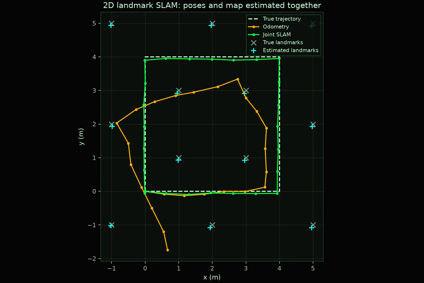
True trajectory (dashed), odometry estimate (orange), and joint SLAM estimate (green); true landmarks (×) and estimated ones (+)
In the chart, the dashed line is the true trajectory, the orange line is the odometry estimate, and the green line is the corrected path. True and estimated landmarks are shown too. The file
results.json keeps the exact values.
These numbers come from a synthetic experiment with specific noise and geometry. You cannot conclude that every real robot will improve by exactly this amount. The point is to see the effect of environment information on path error through a repeatable experiment.
# A More Important Experiment: Remove the Repeated Observations
At the end of the code, we solve the problem one more time — but this time keeping only the first observation of each landmark. The path RMSE in this case is 1.338 m: effectively the odometry error.
The reason is visible in the model: a landmark observed only once can sit wherever it is compatible with that single measurement and the robot's current pose. Since we don't know the landmark's coordinates either, this lone observation connects the robot to no other part of the path.
When the same landmark is seen again, you can no longer pick an independent spot for each observation; every observation must be consistent with the coordinates of one fixed landmark. That connection is what helps correct the path.
This experiment removes all repeated observations; so it is not a separate test of a single loop-closure constraint at the end of the path. It measures the effect of observing the environment multiple times.
# What Does This Example Simplify?
This program is a 2D joint-estimation exercise. A few of its assumptions should be kept in mind when interpreting the result:
- Landmark identities are known; automatic matching of image or scan features is not performed.
- Landmarks are static; outliers and occlusion are not simulated.
- Noise is assumed independent and approximately Gaussian, with known uncertainties.
- The problem is solved in batches after all data is collected; the implementation is not real-time.
- The output is a sparse landmark map; it does not produce a full free-space/obstacle map for path planning.
In the real world, sensor calibration, time synchronization of data, outlier detection, and handling moving objects join the problem too. Good optimization cannot by itself fix every wrong measurement.
# What Is the Path From Simulation to a Real Robot?
If you want to learn the concept, start by changing this example. Increase the odometry noise, reduce the sensor accuracy, or lower the number of observed landmarks, and compare the results. Change one factor at a time so the cause of each change in the output stays clear.
For a project with a 2D laser scanner and ROS, the SLAM Toolbox documentation is a practical reference for mapping and localization. For camera work, ORB-SLAM3 ships official examples for monocular, stereo, RGB-D, and visual-inertial configurations. The choice of system should match the project's sensor type, environment, and computing budget.
One practical note: position estimation and map building alone do not solve safe motion. Path planning, moving-obstacle detection, and robot control need other components.
# So How Does a Robot Know Where It Is Without GPS?
The robot estimates its motion, observes the environment, and finds connections between observations. Then it corrects the robot poses and the map together so they fit the data better.
In our exercise, counting motions accumulated error. Seeing the fixed landmarks again added information that made correcting the path possible. That simple idea, together with sensor processing and uncertainty management, is the foundation of many SLAM systems.
takeaway.txt
"Where am I?" and "What does the map look like?" get no answer alone;
SLAM answers them together.
SLAM answers them together.