# From One Equation to a Runnable Procedure
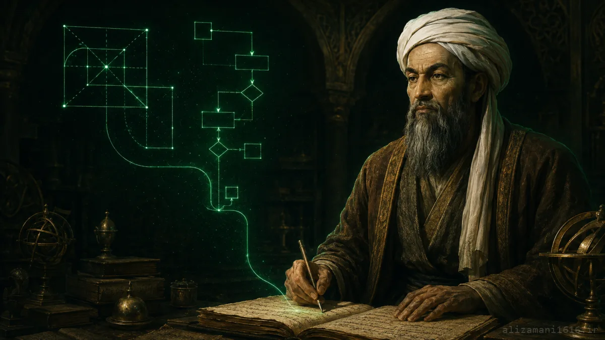
What matters about al-Khwarizmi's work is elsewhere: this Persian scholar presented the solution of linear and quadratic equations in a systematic, teachable, rule-based way. A problem was first reduced to one of a few standard forms, and then the matching solution procedure was executed. In today's software vocabulary, his overall pipeline looks like this:
His method, in software terms
Problem statement
Standardization
Type detection
Method selection
Step-by-step execution
Answer + geometric proof
Two linguistic legacies: the word
algorithm came from the Latinized name of al-Khwarizmi (Algoritmi) in translations of his arithmetic works, while algebra derives from al-jabr in the title of his famous book. One scholar's name became "algorithm", and part of his book's title became the name of a major branch of mathematics.
# How Was a Problem Written Without x or an Equals Sign?
Al-Khwarizmi's book, The Compendious Book on Calculation by Completion and Balancing, explained algebra in prose; the symbolic notation we know today did not yet exist. What we write as:
MODERN
x2
+
10x
=
39
was described in that era with three kinds of quantities:
x²
Square (mal)
What we now call the second power of the unknown
x
Root or thing (shay')
The unknown itself
c
Number
The constant term
The problem statement in the 19th-century translation reads roughly: "A square together with ten of its roots equals thirty-nine; what is that square?" The solution could not be a compact formula — it had to be written as instructions executed in order:
1
Halve the number of roots
2
Multiply the result by itself
3
Add the result to the constant
4
Take the square root of the sum
5
Subtract half the roots
From a programmer's perspective, that text is almost ready to become a function.
# Six Equation Types: Something Like a Type System for Problems
In al-Khwarizmi's system, coefficients and solutions were treated as positive quantities. For that reason, expressions we write today with negative numbers and one general form were split into six separate types:
1
Squares equal roots
ax² = bx2
Squares equal numbers
ax² = c3
Roots equal numbers
bx = c4
Squares and roots equal numbers
ax² + bx = c5
Squares and numbers equal roots
ax² + c = bx6
Roots and numbers equal squares
bx + c = ax²
Modern algebra reduces everything to
ax² + bx + c = 0, but that relies on accepting negative coefficients, zero, and symbolic notation. When all quantities are positive, moving a term to the other side doesn't make it "negative" — it changes the problem's type. From a programming view, al-Khwarizmi's six-item list resembles defining the allowed input states: first detect the pattern, then execute the right branch.
# Al-Jabr and Al-Muqabala: Normalization Before Solving
Before the solution procedure ran, the equation had to be cleaned into one of the standard forms. The two famous operations appear right in the book's title:
al-jabr — completion
A subtracted term is removed by adding the appropriate amount to both sides.
x² = 40x − 4x² → 5x² = 40x
al-muqabala — balancing
Like quantities appearing on both sides are reduced.
50 + 3x + x² = 29 + 10x → 21 + x² = 7x
This stage resembles what a compiler or query optimizer does: inputs may look different, but before the main processing they are transformed into a standard representation:
Normalization
Different problem shapes
al-jabr / al-muqabala
One of six standard forms
A defined solution method
Al-Khwarizmi didn't call it
normalize(), but separating "problem preparation" from "executing the solution" is one of the most familiar patterns in modern software.
# The Main Example: A Square and Ten Roots Equal 39
Back to the opening equation — a type-4 problem: squares and roots equal a number. We execute al-Khwarizmi's method step by step in modern mathematical language:
STEP 1
Halve the roots coefficient
10
2
=
5
STEP 2
Square it
52
=
25
STEP 3
Add to the constant
39
+
25
=
64
STEP 4
Take the root of the sum
√64
=
8
RESULT
x
=
8
−
5
=
3
To verify, substitute back:
3² + 10×3 = 9 + 30 = 39 ✓
Crucially, this sequence wasn't written just for 10 and 39. For the general form
x² + bx = c, the same steps run with inputs b and c:
GENERAL
x
=
√c + (b/2)²
−
b
2
The final formula is a summary of the steps — but the algorithm is the sequence of operations and the conditions under which they run.
# Why Must a Square Be "Completed"?
Following only the numbers, adding 25 might look like a memorized trick. The geometric justification shows where it comes from. Consider
x² as the area of a square with side x. Split 10x into two 5x rectangles and place them along two sides of the square:
x² + 10x + 25 = (x+5)² — the missing corner is exactly 25
geometry.txt
Existing area = x² + 10x = 39
Missing corner = 5² = 25
Full square area = 39 + 25 = 64
Full square side = √64 = 8
Original side = 8 − 5 = 3
This geometric argument doesn't just announce the result; it explains why the steps are correct. In software terms, it is close to a correctness argument for the algorithm: if areas stay equal and the added piece exactly fills the missing corner, the final answer must satisfy the original equation.
# Turning the Verbal Instructions into Pseudocode
ALGORITHM solve_square_and_roots(b, c)
INPUT:
b = number of roots
c = number on the other side
PRECONDITION:
b > 0 and c > 0 and equation is x² + bx = c
STEPS:
half ← b / 2
missing_square ← half × half
completed_area ← c + missing_square
completed_side ← square_root(completed_area)
root ← completed_side − half
OUTPUT:
root
This pseudocode has the core properties of an algorithm: defined inputs, preconditions, clear executable steps, termination after a bounded number of steps, and a defined output. The distance between al-Khwarizmi's text and Python code is now very small.
# First Python Implementation
khwarizmi_basic.py
from math import sqrt
def solve_square_and_roots(b: float, c: float) -> float:
"""Solve x² + bx = c in the positive-number historical setting."""
if b <= 0 or c <= 0:
raise ValueError("b and c must be positive")
half = b / 2
missing_square = half**2
completed_area = c + missing_square
completed_side = sqrt(completed_area)
x = completed_side - half
return x
answer = solve_square_and_roots(10, 39)
print(answer)
$ python khwarizmi_basic.py
3.0
3.0
The variable names deliberately mirror the reasoning steps. The whole function could be one line:
one_liner.py
return sqrt(c + (b / 2) ** 2) - b / 2
But the multi-step version has a teaching advantage: it preserves the structure of the method's thinking. The program doesn't just produce an answer; it shows how the answer is constructed.
# Tracing the Run Like the Historical Text
To see each step, we write a function that returns the computation state along with the answer:
trace_khwarizmi.py
from math import sqrt
def trace_square_and_roots(b: float, c: float) -> dict[str, float]:
if b <= 0 or c <= 0:
raise ValueError("b and c must be positive")
half = b / 2
missing_square = half**2
completed_area = c + missing_square
completed_side = sqrt(completed_area)
x = completed_side - half
return {
"half_of_roots": half,
"missing_square": missing_square,
"completed_area": completed_area,
"completed_side": completed_side,
"answer": x,
}
for step, value in trace_square_and_roots(10, 39).items():
print(f"{step:18} = {value}")
half_of_roots = 5.0
missing_square = 25.0
completed_area = 64.0
completed_side = 8.0
answer = 3.0
missing_square = 25.0
completed_area = 64.0
completed_side = 8.0
answer = 3.0
This trace is a bridge between three representations — changing the language didn't change the step's logic:
1
Historical instruction
"Take half the roots"
2
Modern math
b / 23
Code
half = b / 2# What If the Square's Coefficient Isn't 1?
So far the coefficient of x² was 1. Consider the more general type-4 equation
ax² + bx = c. Before completing the square, we normalize: divide the whole equation by a, then run the same algorithm on the normalized coefficients:
normalized_solver.py
from math import sqrt
def solve_ax2_plus_bx_eq_c(a: float, b: float, c: float) -> float:
"""Solve ax² + bx = c for the positive root."""
if a <= 0 or b <= 0 or c <= 0:
raise ValueError("a, b and c must be positive")
normalized_b = b / a
normalized_c = c / a
half = normalized_b / 2
completed_area = normalized_c + half**2
return sqrt(completed_area) - half
print(solve_ax2_plus_bx_eq_c(2, 20, 78)) # 2x² + 20x = 78 → after /2, same example
3.0
Two independent stages appear here: Normalization (make the square's coefficient 1) and Solution (complete the square). This separation is valuable in software too: the more input shapes exist, the more a canonical internal representation simplifies the solver.
# Building a Solver for All Six Historical Types
Now we go beyond one example and implement all six equation types in one program. It isn't a substitute for a symbolic algebra library; the goal is modeling al-Khwarizmi's system with modern tools:
khwarizmi_solver.py
from __future__ import annotations
from enum import Enum
from math import isclose, sqrt
class EquationType(str, Enum):
SQUARES_EQUAL_ROOTS = "squares_equal_roots"
SQUARES_EQUAL_NUMBERS = "squares_equal_numbers"
ROOTS_EQUAL_NUMBERS = "roots_equal_numbers"
SQUARES_AND_ROOTS_EQUAL_NUMBERS = "squares_and_roots_equal_numbers"
SQUARES_AND_NUMBERS_EQUAL_ROOTS = "squares_and_numbers_equal_roots"
ROOTS_AND_NUMBERS_EQUAL_SQUARES = "roots_and_numbers_equal_squares"
REQUIRED_COEFFICIENTS = {
EquationType.SQUARES_EQUAL_ROOTS: ("a", "b"),
EquationType.SQUARES_EQUAL_NUMBERS: ("a", "c"),
EquationType.ROOTS_EQUAL_NUMBERS: ("b", "c"),
EquationType.SQUARES_AND_ROOTS_EQUAL_NUMBERS: ("a", "b", "c"),
EquationType.SQUARES_AND_NUMBERS_EQUAL_ROOTS: ("a", "b", "c"),
EquationType.ROOTS_AND_NUMBERS_EQUAL_SQUARES: ("a", "b", "c"),
}
def _positive_unique(values: list[float]) -> list[float]:
"""Keep positive roots and remove near-duplicates."""
result: list[float] = []
for value in sorted(values):
if value <= 0:
continue
if not any(isclose(value, old, rel_tol=1e-12) for old in result):
result.append(value)
return result
khwarizmi_solver.py — continued
def solve_historical(equation_type: EquationType, *, a=None, b=None, c=None):
"""Solve one of al-Khwarizmi's six standard equation types."""
values = {"a": a, "b": b, "c": c}
for name in REQUIRED_COEFFICIENTS[equation_type]:
if values[name] is None or values[name] <= 0:
raise ValueError(f"{name} must be a positive number")
if equation_type is EquationType.SQUARES_EQUAL_ROOTS:
# ax² = bx → x = b/a
return [b / a]
if equation_type is EquationType.SQUARES_EQUAL_NUMBERS:
# ax² = c → x = √(c/a)
return [sqrt(c / a)]
if equation_type is EquationType.ROOTS_EQUAL_NUMBERS:
# bx = c → x = c/b
return [c / b]
normalized_b = b / a
normalized_c = c / a
half = normalized_b / 2
if equation_type is EquationType.SQUARES_AND_ROOTS_EQUAL_NUMBERS:
# ax² + bx = c
return _positive_unique([sqrt(normalized_c + half**2) - half])
if equation_type is EquationType.SQUARES_AND_NUMBERS_EQUAL_ROOTS:
# ax² + c = bx — can yield two answers
remaining_square = half**2 - normalized_c
if remaining_square < 0:
return []
distance = sqrt(remaining_square)
return _positive_unique([half - distance, half + distance])
if equation_type is EquationType.ROOTS_AND_NUMBERS_EQUAL_SQUARES:
# bx + c = ax²
return _positive_unique([half + sqrt(normalized_c + half**2)])
raise ValueError(f"Unsupported equation type: {equation_type}")
Now we test all six types with their own examples:
run_examples.py — output
# type 1: x² = 5x
squares_equal_roots → [5.0]
# type 2: x² = 9
squares_equal_numbers → [3.0]
# type 3: 3x = 12
roots_equal_numbers → [4.0]
# type 4: x² + 10x = 39
squares_and_roots_equal_numbers → [3.0]
# type 5: x² + 21 = 10x
squares_and_numbers_equal_roots → [3.0, 7.0]
# type 6: 3x + 4 = x²
roots_and_numbers_equal_squares → [4.0]
The program uses several familiar computer-science ideas: an
Enum defining exactly six valid states; a REQUIRED_COEFFICIENTS table holding each state's input contract; upfront input validation; one branch per rule; and outputs restricted to positive real roots to stay faithful to the historical framework.
This code is not a literal transcription of a manuscript. Enums, floats,
sqrt(), and even comment symbols are modern tools. What has been recreated is the order of decision-making and the computation method.
# Why Can Type 5 Have Two Answers?
The equation
x² + 21 = 10x is another classic of this tradition. Half the roots is 5; its square is 25. This time we subtract: 25 − 21 = 4. The root of 4 is 2, so x = 5 − 2 = 3 — but a second answer exists: x = 5 + 2 = 7. Both satisfy the equation:
verify.txt
3² + 21 = 30 = 10(3) ✓
7² + 21 = 70 = 10(7) ✓
That's why
solve_historical() returns list[float] instead of a single number. This design keeps the output shape uniform across zero-answer, one-answer, and two-answer cases:
output_contract.txt
[] → no positive real answer
[3.0] → one positive answer
[3.0, 7.0]→ two positive answers
Choosing the right data structure is part of turning a mathematical method into software — even when the computation itself is only a few lines.
# Where Did the Negative Answer Go?
Write the main equation in modern form:
x² + 10x − 39 = 0. The quadratic formula gives two answers: x = 3 and x = −13. The historical solver returns only 3. That isn't a bug — it's part of the model we chose. In al-Khwarizmi's framework, "root", "square" and "number" were positive quantities, and a negative answer didn't count as a valid solution.
The same applies to
ax² = bx. Modern algebra says x(ax−b) = 0, so x = 0 or x = b/a. Our historical solver keeps only b/a, because zero also played no role as an answer in that formulation.
A programming lesson: correctness is always measured against the specification. If the spec says "positive real roots in six historical forms", dropping zero and negatives is expected behavior. If the goal were "all complex roots of a polynomial", the same program would be incomplete.
Historical model
Input form: one of six types | negative coefficients and zero/negative/complex answers: absent | explanation: verbal rule and geometry
Modern solver
Input form: ax² + bx + c = 0 | negative coefficients and zero/negative/complex answers: supported | explanation: general symbolic formula
The modern version has a larger domain, but the historical version teaches something else: how to turn a problem into a teachable, repeatable procedure before compact notation exists.
# Algorithm vs Formula
A formula is a compact relation, but a real program must answer more questions: where does the input come from? Are the coefficients valid? Which type is the equation? What if the expression under the root goes negative? One answer or two? Are zero and negatives allowed? What numeric type do we use? How do we test the result? An algorithm isn't just "the mathematical relation" — it's the contract for executing that relation.
For example, in type 5 this condition must be checked before
sqrt():
PRECONDITION — TYPE 5
b
2a
2
−
c
a
≥
0
If it fails, there is no answer in the real domain. In code, that condition becomes a branch:
branch.py
remaining_square = half**2 - normalized_c
if remaining_square < 0:
return [] # no positive real answer
Mathematics defines which states are possible; programming defines how software represents them.
# How Do We Know the Code Actually Works?
Seeing
3.0 isn't enough. Two kinds of tests are possible: testing known examples, and substituting answers back into the equation:
test_khwarizmi.py
from math import isclose
def residual_ax2_plus_bx_eq_c(a, b, c, x) -> float:
return a * x**2 + b * x - c
x = solve_historical(EquationType.SQUARES_AND_ROOTS_EQUAL_NUMBERS, a=1, b=10, c=39)[0]
assert isclose(x, 3.0)
assert isclose(residual_ax2_plus_bx_eq_c(1, 10, 39, x), 0.0, abs_tol=1e-12)
assert solve_historical(EquationType.SQUARES_AND_NUMBERS_EQUAL_ROOTS, a=1, b=10, c=21) == [3.0, 7.0]
assert solve_historical(EquationType.ROOTS_AND_NUMBERS_EQUAL_SQUARES, a=1, b=3, c=4) == [4.0]
In general float computations, prefer
math.isclose() over direct equality, since binary representation of some decimals is inexact. For symbolic or exact-fraction work, tools like fractions.Fraction or decimal.Decimal fit better. The program in this article is educational; production numerical software needs a precisely defined numeric domain, rounding behavior, and boundary handling.
# Which Parts of His Method Resemble Modern Programming?
The main resemblance isn't in how formulas look — it's in how problem-solving is organized:
01
Classification
Before solving, a problem belongs to one of six types — like a parser or validation layer detecting the input shape
02
Normalization
Extra terms removed, square coefficient set to 1 — like canonicalizing varied inputs
03
Dispatch
The equation type selects the rule — like if/match or a dispatch table
04
Visible State
Each step produces an intermediate value — exactly what helps debugging and tracing
05
Preconditions
Each method is valid only on specific forms; the right formula on the wrong input still yields wrong answers
06
Correctness Argument
The geometric proof explains why the steps preserve equality — good algorithms come with a reason to trust the output
07
Reuse
The rule isn't tied to one number; any equation meeting the preconditions runs through the same steps
# Can We Call Al-Khwarizmi "The Inventor of the Algorithm"?
The phrase is appealing but historically oversimplified. Algorithms as step-by-step procedures predate him; Euclid's GCD method is an earlier example. A more precise account:
1
Al-Khwarizmi presented arithmetic and algebra methods systematically, step by step
2
His arithmetic works influenced the transfer of the Hindu–Arabic numeral system to Europe
3
His Latinized name became a word for computation methods
4
That word's meaning broadened into today's algorithm
So it's more accurate to say his name and works hold a foundational place in the history of computation and in the word "algorithm" — not that he invented the concept of every algorithm from scratch. The same care applies to algebra: he wasn't the first person ever to solve a quadratic; the importance of his book lies in its systematic, general, teachable formulation of equation-solving. This correction doesn't diminish the story — it shows that scientific progress is usually not one magic moment or a lone inventor: existing knowledge gets collected, organized, and extended across generations.
# If Al-Khwarizmi Saw This Function Today, What Would Be Unfamiliar?
Almost all of the syntax: letters as variable names, the equals sign as assignment, the
** power operator, the library function sqrt(), zero and negative coefficients, the float type, and functions/inputs/outputs/exceptions as software concepts. But if we translate each line back into a verbal instruction, the computational core becomes familiar:
translation.txt
b / 2 → take half the number of roots
(b / 2) ** 2 → multiply that value by itself
c + (b / 2) ** 2 → add the square to the number
sqrt(...) → take the root of the sum
... - b / 2 → subtract half the roots
We didn't discover a historical program; we modeled a historical method in today's execution environment. That distinction is the precise meaning of "implementing al-Khwarizmi's method in Python".
# The Final Solution Pipeline
The whole article can be summarized in one pipeline:
Full pipeline
Problem
square + ten roots = 39
square + ten roots = 39
Modern form
x² + 10x = 39
x² + 10x = 39
Classification
type 4
type 4
Normalization
coefficient = 1
coefficient = 1
Algorithm
halve → square → add → root → subtract
halve → square → add → root → subtract
Result + check
x = 3 ✓
x = 3 ✓
Mathematics defines the problem; the algorithm defines the order of solution; and the program turns that order into something a machine can execute.
# He Didn't Write Code, but He Made Problems Runnable
Al-Khwarizmi's legacy isn't just that he solved one particular equation. The more lasting achievement was turning a mass of seemingly different problems into a few known forms and a few repeatable procedures. In the example
x² + 10x = 39, he doesn't ask the reader to guess 3. He gives a path: halve the roots coefficient, square it, add to 39, take the root, subtract the half. Anyone who executes the steps correctly arrives at the same answer, independent of personal intuition.
Today we put that same idea inside a function, wrote a contract for its inputs, defined the states with an Enum, returned the result in a list, and verified it with tests. The tools are new, but the core thinking is familiar: turn problems into clear, repeatable instructions.
He had no computer, yet he wrote a procedure that could be executed.
takeaway.txt
He didn't write code;
he broke the problem into repeatable steps.
he broke the problem into repeatable steps.