How a City Is Simulated on a Computer Before It Is Built - Ali Zamani

# A Question Maps Cannot Answer

Every urban decision — a new street, a traffic signal, a bus line — has a cascade effect. You can't predict that effect by looking at a map, because traffic is the result of thousands of independent driver decisions interacting, not a fixed property of the streets themselves.

The questions we actually need to answer look like this:

Intersections

Does one specific junction lock up?
What happens with new signal timing?

Routes

Does traffic just get displaced?
Which routes will drivers pick?

Stress Conditions

What if it rains?
What if a street closes?

Extra Load

20,000 additional vehicles?
Rush-hour peaks?

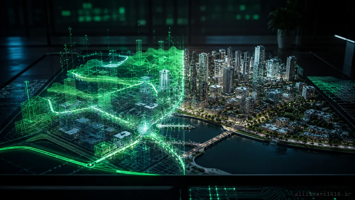
The tool for this job is urban simulation. A serious urban simulator is not just a pretty 3D map: streets, vehicles, signals, routes, and driver behavior are all converted into sets of rules and computations, and the computer advances the city second by second. SUMO — one of the best-known open-source tools in this field — is a microscopic, time-discrete simulator that can model vehicles, pedestrians, public transport, and traffic lights.

# You Cannot Simulate a City All at Once

Let's drop the first misconception: the computer is not going to load "the city" like a 3D game and press Play. A city is not a single entity for a computer — it's a huge network of small systems:

City

An overall system of smaller systems

Streets & Lanes

Each street has multiple lanes with a direction

Intersections & Right-of-Way

Each junction has its own priority and turn rules

Traffic Signals

Phases, timing, and control logic

Vehicles & Pedestrians

Decision-making agents with behavior models

Public Transport

Lines, stops, and schedules

In SUMO, a traffic simulation needs at minimum two things: a road network and travel demand. The network contains roads, lanes, and junctions; the demand specifies which vehicle moves, when, and along which route. So the first step is not "building the cars" — it's building the world the cars will move through.

# Step One: Turning a Real City into a Computable Network

Say we've picked a district of Tehran. What we see on Google Maps isn't enough for a simulator. The computer needs to know which points are intersections, which lines are streets, how many lanes each street has, and which direction each lane runs. This structure maps naturally onto a graph:

Urban Concept	Graph Equivalent	Attached Data
Intersection	Node	Coordinates, priority rules
Street (between two junctions)	Edge	Length, speed limit, shape
Lane	Lane	Direction, width, allowed vehicle classes
Junction connection	Connection	Which lane feeds into which lane

Key idea: to a computer, a city is first of all not an image — it's a graph. An entire city becomes one very large graph that we can run computations on.

How do we get the real map into the simulator? SUMO can import OpenStreetMap street data and turn it into a usable network. The official SUMO documentation recommends exactly this path for building an urban scenario: fetch data from OpenStreetMap and convert it into a simulation network.

1

OpenStreetMap — raw street data

2

netconvert — convert to a simulation network

3

city.net.xml — a computable graph

4

sumo-gui — visualize and run

If the network has flaws, netedit lets you fix them: lane counts, directions, signals, turn restrictions, and banned routes. SUMO's own scenario-building docs warn that networks imported from raw data can contain defects, and junctions, lanes, and signals may need manual correction. A simulation is only as good as its input data.

# Next Problem: A City Without Cars

If we rebuild the exact streets of the real world but never insert a single car, the city stays perfectly empty. So we need to build Traffic Demand. In its simplest form, demand answers: who starts where and goes where? For thousands of vehicles, these paths become a set of trips. In SUMO you can define demand with Vehicle, Flow, Trip, and Route.

Flow	Origin	Destination	Rate	Vehicle Type
Flow A	edge-east	edge-west	1000 veh/h	Passenger car
Flow B	edge-north	edge-south	700 veh/h	Cars & vans
Flow C	edge-west	edge-north	300 veh/h	Light truck

But not all cars behave the same. A compact car, a truck, a bus, and a motorcycle don't move alike — and even two drivers in identical cars don't necessarily behave identically. So each vehicle can carry properties like Maximum Speed, Acceleration, Deceleration, Length, Vehicle Class, and Preferred Speed. Now when 10,000 vehicles enter the city, we no longer have a simple random motion — every vehicle makes decisions according to a set of rules.

# How Does the Driver Inside the Computer Decide?

The computer doesn't need to simulate a complete human or know "how this driver feels this morning." A behavioral model is enough:

Condition	Model Reaction	Simulation Term
Lead vehicle gets close	Slow down, keep the gap	Car-Following
Light is red	Stop at the stop line	Junction Model
Route ahead is congested	Change lane or find an alternative	Lane-Changing / Re-routing
Oncoming traffic has priority	Yield the right-of-way	Right-of-Way

In microscopic simulations, each vehicle's motion is computed individually. Car-Following models determine vehicle behavior from the gap and speed of the vehicle ahead plus driver characteristics. This means our city is no longer made of thousands of "moving dots" — it's made of thousands of decision-making agents.

# Now the City Starts to "Live"

Suppose the simulation runs with a one-second time step. SUMO executes simulations with a one-second step length by default, though the step size is configurable. Each step repeats this cycle:

1

Read state — position & speed of every vehicle

2

Driver decisions — accelerate, brake, change lanes

3

Update signals — switch phases at the right instant

4

Move — new position & speed for every vehicle

↻

Next step — t = t + 1 until the simulation ends

With 10,000 vehicles, the computer must compute the state of a large number of them at every instant. Which is exactly why "not every part of a city is simulated at the same level of detail" — and that's the next topic.

# Fidelity Levels: From Flow to Engine Internals

You might assume a realistic simulation must compute every movement of every vehicle precisely. But that's not always necessary. Traffic simulation typically comes in several levels of detail, and the SUMO documentation separates exactly these levels:

Macroscopic

Instead of individual cars, traffic flow is modeled — e.g. 700 vehicles per hour on a lane.

Compute cost: low

Mesoscopic

A mix of flow and individual behavior; vehicles move through "cells" of the network.

Compute cost: medium

Microscopic

Every vehicle is modeled individually — SUMO's default level for urban scenarios.

Compute cost: high

Sub-microscopic

Internal vehicle details enter the model too — engine or braking dynamics, for example.

Compute cost: very high

Golden rule: a good simulation is not necessarily the most accurate one — it's the one that answers the right question at the right level. If you're studying a new highway's effect on the whole city, you probably don't need to model each car's engine.

# Now Let's Ask a Real Question

Suppose we want to know what closing a main street does. We build two versions of the city — the current one, and one where the A → B link is closed — and run both with identical demand:

Metric

Street Open

Street Closed

Average travel time

8.2 min

11.6 min

Average speed

31 km/h

22 km/h

Waiting time at junction C

24 s

71 s

Queue length on the detour

~40 m

~180 m

Extra delay distribution after closing the street (sample scenario)

Junction C

+47 s

Detour route

+33 s

Northern highway

+14 s

Southern local streets

+6 s

Numbers are a hypothetical scenario illustrating the comparison method; in a real project these values are extracted from simulation output.

This is where simulation truly earns its value: we're no longer watching an animation — we're comparing two possible futures.

# A New Street Doesn't Always Reduce Traffic

This is the most interesting part. Suppose we built a new street to reduce congestion in a district. At first glance the answer should be positive. But a large number of drivers may switch to the shorter route, and the outcome reverses:

New street

→

Attracts more drivers

→

Higher demand

→

Congestion elsewhere

↺ the cycle repeats

Traffic research even has a name for this problem: User Assignment. When every driver chases their own personal best route, the sum of those individual choices can produce severe congestion on some links. SUMO provides Dynamic User Assignment models for exactly this problem. In other words: the best route for one driver is not necessarily the best outcome for a city — one of the key differences between "individual optimization" and "system optimization."

# A Traffic Signal Is a System of Its Own

Take a four-way intersection. The signal can run different timing plans, and each change reshapes the whole junction's behavior:

Plan 1 — Symmetric

NS 30s

4s

EW 30s

Equal green for both axes; suits intersections with symmetric demand.

Plan 2 — Asymmetric

NS 45s

4s

EW 15s

More green for the busy axis; the light axis's queue grows longer.

SUMO lets you model real signals in detail and even attach custom signal-control algorithms to the simulation. So we can genuinely experiment: what is the best timing for this signal at this intersection?

# This Is Where Python Comes In

SUMO isn't just a graphical application. Through TraCI we can communicate with it while the simulation runs. TraCI is a TCP interface that lets an external program read object states and change their behavior mid-run:

Python

↔

TraCI (TCP)

↔

SUMO

↔

City Simulation

That means we can write a program that runs the simulation, reads vehicle counts and queue lengths, changes the signal, and inspects the result again. This is no longer an animation — it's a programmable scientific experiment. For example, a simple adaptive signal controller:

adaptive_signal.py

import traci

traci.start(["sumo", "-c", "city.sumocfg"])

while traci.simulation.getMinExpectedNumber() > 0:
    # read queue lengths on both axes of the junction
    q_ns = sum(traci.lane.getLastStepHaltingNumber(lane)
               for lane in ["n_0", "s_0"])
    q_ew = sum(traci.lane.getLastStepHaltingNumber(lane)
               for lane in ["e_0", "w_0"])

    # give the busier axis more green
    if q_ns > q_ew:
        traci.trafficlight.setPhase("junction_C", 0)  # NS green
    else:
        traci.trafficlight.setPhase("junction_C", 2)  # EW green

    traci.simulationStep()

traci.close()

This same idea can be combined with more sophisticated algorithms — or even AI. In that case a feedback loop forms:

Traffic Data

→

Controller

→

Traffic Light

→

New Traffic State

↺ back to the controller

# And Suddenly We Can Bring AI Into the City

Suppose we want the best signal timing. We can run thousands of configurations and measure travel time, waiting time, queue length, fuel consumption, and emissions for each. Then an optimization algorithm or AI searches for the combination with the best result. The city becomes a laboratory for algorithms:

Scenario	Green NS / EW	Travel Time	Waiting	Max Queue
#1	30s / 30s	11.6 min	96 s	180 m
#2	40s / 20s	10.4 min	78 s	142 m
#3	45s / 15s	9.8 min	61 s	118 m
#4	50s / 10s	12.9 min	124 s	205 m

Note: scenario #4 gives the busy axis even more green, yet performs worse — because the light axis effectively locks up. These are exactly the kinds of insights that only emerge from running a simulation many times.

# Calibrating the City with Real Data

Suppose we have real-world counts but our model says something else. Our model is too optimistic, and we adjust parameters until it tracks reality more closely. This process is Calibration:

Vehicles entering the district — real data vs initial model

08:00 — Real

3200

08:00 — Model

2500

08:15 — Real

4700

08:15 — Model

3900

08:30 — Real

6200

08:30 — Model

5100

The initial model underestimates reality in every interval; demand and behavior parameters must be corrected.

Real City

→

Real Data

→

Simulation

→

Compare

→

Adjust Model

↺ repeat until convergence

This part matters enormously: a good digital city doesn't merely "look realistic" — it must be able to reproduce the observed behavior of the real city.

# This Is Exactly Where the Digital Twin Begins

If we've only built a hypothetical city, we have a Simulation. But if the digital model stays continuously connected to the real city and receives real data, we enter the territory of the Digital Twin:

Simulation

Static model with fixed inputs

Built and run once
Answers "what-if" questions
Used for scenario comparison

Digital Twin

Living model connected to the real city

Receives live data from sensors
Continuously recalibrated
Used for real-time and long-term decisions

Recent research on Urban Digital Twins focuses precisely on this connection to dynamic data, because a static model cannot represent a city that changes constantly. Mobile crowdsourced data and other moving sources are among the ways to add this dynamism.

# But Why Simulate Humans at All?

One of the newest lines of urban research focuses exactly here. In June 2026, a study in npj Complexity presented an Agent-Based framework for simulating urban life patterns, modeling people's daily schedules as a combination of mandatory activities like work and school and flexible activities like shopping and leisure, then validating the results against real travel data. The attractive idea: instead of saying "100,000 trips," we say:

Agent	Daily Schedule	Trips Produced
Person 1	Home → Work → Shopping → Home	3 trips
Person 2	Home → School → Home	2 trips
Person 3	Home → Work → Gym → Home	3 trips

Then the collective behavior of these individuals generates the urban patterns. Traffic may be a large-scale phenomenon at the city level, but it can be built from the sum of thousands of small human decisions.

# One Crucial Caveat: Simulation Does Not See the Future

This may be the most scientifically important part of this post. Simulation is not prophecy. If the model mispredicts tomorrow's city, that doesn't necessarily mean the software is broken:

Bad Input

Outdated or incomplete demand data

Changed Behavior

People's travel patterns shifted

Oversimplified Model

Unrealistic behavioral assumptions

Out-of-Model Event

Something the model never contained

So what's the correct formula? Simulation ≠ Future. Simulation = "if these assumptions hold, this will probably happen." That difference is the border between a scientific model and fortune-telling. The main enemy of simulation is not model simplicity — it's trusting a model that has never been validated.

# Why a Simple Model Sometimes Beats a Complex One

Imagine we want to know how a new street affects travel time. We don't need to simulate the engine, model the tires, or compute combustion. This principle matters a lot in simulation: compute the details that matter for your question. That's why a good urban simulation is not necessarily the one with the most detail — it's the one that answers the right question at an acceptable cost.

Question	Suitable Level	Why
Effect of a new highway on the whole city	Macro / Meso	Large scale; individual detail irrelevant
Timing of one specific signal	Micro	Queue behavior and start-up dynamics matter
Energy use of an electric fleet	Sub-micro	Vehicle dynamics enter the computation

# If We Really Wanted to Design a Future City

The full path of a serious urban simulation project looks something like this:

1

OpenStreetMap — the real district map

2

Road network — a computable graph

3

Demand & vehicle models — trips and properties

4

Simulation — step-by-step execution

5

Calibration — close the gap to real data

6

AI / Optimization — search for the best scenario

And if this system connects to the city's live data, the loop closes: sensors produce data, the Digital Twin stays current, the simulation tests scenarios, a decision is made, and the outcome flows back into the model. At this point we're no longer dealing with a "3D map of the city" — we're dealing with a computational copy of the city.

# We Don't Build the City; We Test Its Hypothesis First

Back to the original question: how do they run a city on a computer before building it? Not by making a computer game of the city — by building a computational model. Streets become a network, cars become agents, drivers are approximated with behavioral models, signals become timing and control rules, and the population becomes travel patterns. Then we run hours, days, and whole scenarios to see how the system reacts when conditions change.

The traditional way: idea → build → observe the result. The data-driven way: idea → simulation → hundreds of scenarios → choose → build → measure → feed data back into the model. Before an urban decision carries a real-world cost, its digital version can be tested — and after construction, the work isn't over, because the real city produces data and the model keeps getting corrected.

takeaway.txt

              The future of urban planning is not building the city first and seeing what happens.

              The future is simulating a thousand versions of a city in the computer before building it —

              crafting a fresh scenario with each small change, and finally bringing only the best version into the real world.